How to find the number of physical CPUs in Linux

1. How many physical CPUs does the server have?
2. How many cores on each CPU? Duo/Quad

In Linux it’s actually quite easy to get this info.
You could go through the /var/log/dmesg file or the /proc/cpuinfo file. We’ll look at the /proc/cpuinfo file.

Output of cat /proc/cpuinfo:
processor : 0
vendor_id : GenuineIntel
cpu family : 6
model : 26
model name : Intel(R) Xeon(R) CPU X5570 @ 2.93GHz
stepping : 5
cpu MHz : 2933.548
cache size : 8192 KB
physical id : 1
siblings : 8
core id : 0
cpu cores : 4
apicid : 16
fpu : yes
fpu_exception : yes
cpuid level : 11
wp : yes

flags : fpu vme de pse tsc msr pae mce cx8 apic sep mtrr pge mca cmov pat pse36 clflush dts acpi mmx fxsr sse sse2 ss ht tm syscall nx rdtscp lm constant_tsc nonstop_tsc pni monitor ds_cpl vmx est tm2 ssse3 cx16 xtpr sse4_1 sse4_2 popcnt lahf_lm
bogomips : 5867.09
clflush size : 64
cache_alignment : 64
address sizes : 40 bits physical, 48 bits virtual
power management: [8]
processor : 1
vendor_id : GenuineIntel
cpu family : 6
model : 26
model name : Intel(R) Xeon(R) CPU X5570 @ 2.93GHz
stepping : 5
cpu MHz : 2933.548
cache size : 8192 KB
physical id : 0
siblings : 8
core id : 0
cpu cores : 4
apicid : 0
fpu : yes
fpu_exception : yes
cpuid level : 11
wp : yes
flags : fpu vme de pse tsc msr pae mce cx8 apic sep mtrr pge mca cmov pat pse36 clflush dts acpi mmx fxsr sse sse2 ss ht tm syscall nx rdtscp lm constant_tsc nonstop_tsc pni monitor ds_cpl vmx est tm2 ssse3 cx16 xtpr sse4_1 sse4_2 popcnt lahf_lm
bogomips : 5866.85
clflush size : 64
cache_alignment : 64
address sizes : 40 bits physical, 48 bits virtual
power management: [8]

1. To get Physical CPU count?
Run “cat /proc/cpuinfo | grep “physical id” | sort | uniq | wc -l”.
$ cat /proc/cpuinfo | grep "physical id" | sort | uniq|wc -l
Output : 2
The machine has two Physical CPU.

2. How many cores?
Run “cat /proc/cpuinfo | grep “cpu cores” | uniq”.
$ cat /proc/cpuinfo | grep "cpu cores" | uniq
Output: cpu cores : 4
The machine has four Cores
4 mean that each physical CPU has 4 cores on it. If cpu cores was 1 then the CPU’s single core.

How many virtual processors?

Run “cat /proc/cpuinfo | grep “^processor”"
$ cat /proc/cpuinfo | grep "^processor"
processor : 0
processor : 1
processor : 2
processor : 3
processor : 4
processor : 5
processor : 6
processor : 7
processor : 8
processor : 9
processor : 10
processor : 11
processor : 12
processor : 13
processor : 14
processor : 15
We have 2 physical CPUs x 4 cores each = 8 virtual processors. So there should be 8 Virtual Processors. But here the Output is 16. Why is it showing 16.

The processor number is showing 16, due to HT (Hyper-Threading) enablement.

However, it’s a bit different for HT (Hyper-Threading). If you get cpu core = 1 but the virtual processors = 2 then the CPU’s running HT. HT will only work with the SMP kernel.

Parameterization in Jmeter

Parameterization in Jmeter:

We parameterize the input to run the test with different set of data for each user. We will provide the data in a file and provide as input for a field.

For this we will create a .csv file in Excel and save it. For this example, we will parameterize four fields. They are fromPort, toPort, passFirst0 and passLast0.

 The details to corresponding fields are as follows:

We have our requests as shown below:

To add the data to the test we need to add the config element as below:

Right Click on Thread Group -> Add -> Config Element -> CSV Data Set Config

The CSV Data Set details were entered as follows:

Parameters for the CSV Data Set config is as below:

Attribute Description Required Name Descriptive name for this element that is shown in the tree. No Filename Name of the file to be read. Relative file names are resolved with respect to the path of the active test plan. Absolute file names are also supported, but note that they are unlikely to work in remote mode, unless the remote server has the same directory structure. If the same physical file is referenced in two different ways - e.g. csvdata.txt and ./csvdata.txt - then these are treated as different files. If the OS does not distinguish between upper and lower case, csvData.TXT would also be opened separately. Yes File Encoding The encoding to be used to read the file, if not the platform default. No Variable Names List of variable names (comma-delimited). Versions of JMeter after 2.3.4 support CSV header lines: if the variable name field empty, then the first line of the file is read and interpreted as the list of column names. The names must be separated by the delimiter character. They can be quoted using double-quotes. Yes Delimiter Delimiter to be used to split the records in the file. If there are fewer values on the line than there are variables the remaining variables are not updated - so they will retain their previous value (if any). Yes Allow quoted data? Should the CSV file allow values to be quoted? If enabled, then values can be enclosed in " - double-quote - allowing values to contain a delimeter. Yes Recycle on EOF? Should the file be re-read from the beginning on reaching EOF? (default is true) Yes Stop thread on EOF? Should the thread be stopped on EOF, if Recycle is false? (default is false) Yes Sharing mode All threads - (the default) the file is shared between all the threads. Current thread group - each file is opened once for each thread group in which the element appears Current thread - each file is opened separately for each thread Identifier - all threads sharing the same identifier share the same file. So for example if you have 4 thread groups, you could use a common id for two or more of the groups to share the file between them. Or you could use the thread number to share the file between the same thread numbers in different thread groups.

Now once the CSV Data Set is configured, we need to set the variables at appropriate position as shown:

The value is set as ${Variablename} for the required fields. For example here passFirst0 is set as ${FirstName} and passLast0 is set as ${LastName}.

Let us now verify the values are passed correctly to the required parameters from the csv file. To perform this we will add a Listener -> View Results tree as below:

In Thread group set the Number of users as 2 and run. We see that there are two sample results as we ran for two users. We check the first thread we see that fromPort is Frankfurt and toPort is London which is same as first record of our .csv file.

Now, let us verify the second thread results, we see that fromPort is London and toPort is New York. So for two different customers there are two different input provided.

In the same way we can check for the customer firstname and lastname also.

We can define one file and all requests can use same file for the parameters. In this way we can parameterize the data in Jmeter.

Performance Testing Concepts

Performance Testing : There are lot of Definitions available but the one mentioned in IEEE Glossary is as follows:

“Testing conducted to evaluate the compliance of a system or component with specified performance requirements. Often this is performed using an automated test tool to simulate large number of users. Also known as "Load Testing".

Or

“The testing performed to determine the degree to which a system or component accomplishes its designated functions within given constraints regarding processing time and throughput rate.”

The purpose of the test is to measure characteristics, such as response times, throughput or the mean time between failures (for reliability testing)

Performance testing tool:A tool to support performance testing and that usually has two main facilities: load generation and test transaction measurement. Load generation can simulate either multiple users or high volumes of input data. During execution, response time measurements are taken from selected transactions and these are logged. Performance testing tools normally provide reports based on test logs and graphs of load against response times.

Features or characteristics of performance-testing tools include support for:
• generating a load on the system to be tested;
• measuring the timing of specific transactions as the load on the system varies;
• measuring average response times;
• producing graphs or charts of responses over time.

Load test:
A test type concerned with measuring the behavior of a component or system with increasing load, e.g. number of parallel users and/or numbers of transactions to determine what load can be handled by the component or system

While doing Performance testing we measure some of the following:

1. Characterisitics (SLA) Measurement (units)
2. Response Time Seconds
3. Hits per Second #Hits
4. Throughput Bytes Per Second
5. Transactions per Second (TPS) #Transactions of a Specific Business Process
6. Total TPS (TTPS) Total no.of Transactions
7. Connections per Second (CPS) #Connections/Sec
8. Pages Downloaded per Second (PDPS) #Pages/Sec

The objective of a performance test is to ensure that the application is working perfectly under load. However, the definition of “perfectly” under load may vary with different systems.
By defining an initial acceptable response time, we can benchmark the application if it is performing as anticipated.

The importance of Transaction Response Time is that it gives the project team/ application team an idea of how the application is performing in the measurement of time. With this information, they can relate to the users/customers on the expected time when processing request or understanding how their application performed.

What does Transaction Response Time encompass?
The Transaction Response Time encompasses the time taken for the request made to the web server, there after being process by the Web Server and sent to the Application Server. Which in most instances will make a request to the Database Server. All this will then be repeated again backward from the Database Server, Application Server, Web Server and back to the user. Take note that the time taken for the request or data in the network transmission is also factored in.


To simplify, the Transaction Response Time comprises of the following:
1. Processing time on Web Server
2. Processing time on Application Server
3. Processing time on Database Server.
4. Network latency between the servers, and the client.


The following diagram illustrates Transaction Response Time.


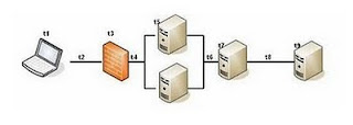
Transaction Response Time = (t1 + t2 + t3 + t4 + t5 + t6 + t7 + t8 + t9) X 2
Note:
Factoring the time taken for the data to return to the client.

How do we measure?

Measuring of the Transaction Response Time begins when the defined transaction makes a request to the application. From here, till the transaction completes before proceeding with the next subsequent request (in terms of transaction), the time is been measured and will stop when the transaction completes.

Differences with Hits Per Seconds
Hits per Seconds measures the number of “hits” made to a web server. These “hits” could be a request made to the web server for data or graphics. However, this counter does not represent well to users on how well their applications is performing as it measures the number of times the web server is being accessed.

How can we use Transaction Response Time to analyze performance issue?
Transaction Response Time allows us to identify abnormalities when performance issues surface. This will be represented as slow response of the transaction, which differs significantly (or slightly) from the average of the Transaction Response Time.
With this, we can further drill down by correlation using other measurements such as the number of virtual users that is accessing the application at the point of time and the system-related metrics (e.g. CPU Utilization) to identify the root cause.
Bringing all the data that have been collected during the load test, we can correlate the measurements to find trends and bottlenecks between the response time, the amount of load that was generated and the payload of all the components of the application.

How is it beneficial to the Project Team?
Using Transaction Response Time, Project Team can better relate to their users using transactions as a form of language protocol that their users can comprehend. Users will be able to know that transactions (or business processes) are performing at an acceptable level in terms of time.
Users may be unable to understand the meaning of CPU utilization or Memory usage and thus using a common language of time is ideal to convey performance-related issues.

Relation between Load, Response Time and Performance:
1. Load is Directly Proportional to Response Time
2. Performance is inversely proportional to Response Time.

So, As and When the Load increases the Response Time Increases. As Response Time Increases, the Performance Decreases.

Hits Per Second
A Hit is a request of any kind made from the virtual client to the application being tested (Client to Server). It is measured by number of Hits. The higher the Hits Per Second, the more requests the application is handling per second.

A virtual client can request an HTML page, image, file, etc. Testing the application for Hits Per Second will tell you if there is a possible scalability issue with the application. For example, if the stress on an application increases but the Hits Per Second does not, there may be a scalability problem in the application.

One issue with this metric is that Hits Per Second relates to all requests equally.
Thus a request for a small image and complex HTML generated on the fly will both be considered as hits. It is possible that out of a hundred hits on the application, the application server actually answered only one and all the rest were either cached on the web server or other caching mechanism.

So, it is very important when looking at this metric to consider what and how the
application is intended to work. Will your users be looking for the same piece of
information over and over again (a static benefit form) or will the same number of users be engaging the application in a variety of tasks – such as pulling up images, purchasing items, bringing in data from another site? To create the proper test, it is important to understand this metric in the context of the application. If you’re testing an application function that requires the site to ‘work,’ as opposed to present static data, use the pages per second measurement.

Pages Per Second
Pages Per Second measures the number of pages requested from the application per second. The higher the Page Per Second the more work the application is doing per second. Measuring an explicit request in the script or a frame in a frameset provides a metric on how the application responds to actual work requests. Thus if a script contains a Navigate command to a URL, this request is considered a page. If the HTML that returns includes frames they will also be considered pages, but any other elements retrieved such as images or JS Files, will be considered hits, not pages. This measurement is key to the end-user’s experience of application performance.

Correlation: If the stress increases, but the Page Per Second count doesn’t, there may be a scalability issue. For example, if you begin with 75 virtual users requesting 25 different pages concurrently and then scale the users to 150, the Page Per Second count should increase. If it doesn’t, some of the virtual users aren’t getting their pages. This could be caused by a number of issues and one likely suspect is throughput.

Throughput
“The amount of data transferred across the network is called throughput. It considers the amount of data transferred from the server to client only and is measured in Bytes/sec.”

This is an important baseline metric and is often used to check that the application and its server connection is working. Throughput measures the average number of bytes per second transmitted from the application being tested to the virtual clients running the test agenda during a specific reporting interval. This metric is the response data size (sum) divided by the number of seconds in the reporting interval.

Generally, the more stress on an application, the more Throughput. If the stress increases, but the Throughput does not, there may be a scalability issue or an application issue.

Another note about Throughput as a measurement – it generally doesn’t provide any information about the content of the data being retrieved. Thus it can be misleading especially in regression testing. When building regression tests, leave time in the testing plan for comparing returned data quality.

Round Trips

Another useful scalability and performance metric is the testing of Round Trips. Round Trips tells you the total number of times the test agenda was executed versus the total number of times the virtual clients attempted to execute the Agenda. The more times the agenda is executed, the more work is done by the test and the application.
The test scenario the agenda represents influences the round Trips measurement.
This metric can provide all kinds of useful information from the benchmarking of an application to the end-user availability of a more complex application. It is not
recommended for regression testing because each test agenda may have a different scenario and/or length of scenario.

Hit Time:

Hit time is the average time in seconds it took to successfully retrieve an element of any kind (image, HTML, etc). The time of a hit is the sum of the Connect Time, Send Time, Response Time and Process Time. It represents the responsiveness or performance of the application to the end user. The more stressed the application, the longer it should take to retrieve an average element. But, like Hits Per Second, caching technologies can influence this metric. Getting the most from this metric requires knowledge of how the application will respond to the end user.
This is also an excellent metric for application monitoring after deployment.

Time to First Byte
This measurement is important because end users often consider a site malfunctioning if it does not respond fast enough. Time to First Byte measures the number of seconds it takes a request to return its first byte of data to the test software’s Load Generator.
For example, Time to First Byte represents the time it took after the user pushes the “enter” button in the browser until the user starts receiving results. Generally, more concurrent user connections will slow the response time of a request. But there are also other possible causes for a slowed response.
For example, there could be issues with the hardware, system software or memory issues as well as problems with database structures or slow-responding components within the application.

Page Time
Page Time calculates the average time in seconds it takes to successfully retrieve a page with all of its content. This statistic is similar to Hit Time but relates only to pages. In most cases this is a better statistic to work with because it deals with the true dynamics of the application. Since not all hits can be cached, this data is more helpful in terms of tracking a user’s experience (positive or frustrated). It’s important to note that in many test software application tools you can turn caching on or off depending on your application needs.

Generally, the more stress on the site the slower its response. But since stress is a combination of the number of concurrent users and their activity, greater stress may or may not impact the user experience. It all depends upon the application’s functions and users. A site with 150 concurrent users looking up benefit information will differ from a news site during a national emergency. As always, metrics must be examined within context.

Failed Rounds/Failed Rounds Per Second

During a load test it’s important to know that the application requests perform as
expected. The Failed Rounds and Failed Rounds Per Second tests the number of
rounds that fail.

This metric is an “indicator metric” that provides QA and test with clues to the
application performance and failure status. If you start to see Failed Rounds or Failed Rounds Per Second, then you would typically look into the logs to see what types of failures correspond to this metric report. Also, with some software test packages, you can set what the definition of a failed round in an application.

Sometimes, basic image or page missing errors (HTTP 404 error codes) could be set to fail a round, which would stop the execution of the test agenda at that point and start at the top of the agenda again, thus not completing that particular round.

Failed Hits/Failed Hits Per Second
This test offers insight into the application’s integrity during the load test. An example of a request that might fail during execution is a broken link or a missing image from the server. The number of errors should grow with the load size. If there are no errors with a low load, the number of errors with a high load should remain zero. If the percentage of errors only increases during high loads, the application may have a scalability issue.

Failed Connections
This test is simply the number of connections that were refused by the application during the test. This test leads to other tests. A failed connection could mean the server was too busy to handle all the requests, so it started refusing them. It could be a memory issue. It could also mean that the user sent bogus or malformed data to which the server couldn’t respond so it refused the connection.

Loadrunner MAPI Protocol

The comments made here about the Loadrunner MAPI protocol are applicable for Loadrunner version 8.1. MAPI is Loadrunner’s Microsoft Exchange protocol.

I had reasonably straight forward objectives for a test I was preparing. Ramp up a few hundred users who would simulate use of Microsoft Exchange, i.e. users who were logging on, sending and receiving emails

I expected that Loadrunner would work with Outlook much like Loadrunner works with Internet Explorer. Loadrunner can simulate Internet Explorer with multiple users and sessions all working independently. Whilst working with the MAPI protocol I discovered that Loadrunner struggles to interact with Outlook. Some of the problems encountered were:


1) Not all of the statements worked. While they did not cause any problems, they just did not do what they were supposed to do. For instance:

The following statement should return a message ID, which it didn’t.

msgid = mapi_get_property_sz_ex(&mapi, "Message ID");

The following statement deleted a mail, but would not delete another email unless the logon statement was reissued on a fresh iteration:

mapi_delete_mail_ex(&mapi,"NextMail", "Show=all", LAST);

2) While the logon statement worked, it was not possible to logon a user to Outlook unless that user was logged onto the domain. Theoretically, the web_set_user will do this for you but it was not possible to introduce a web statement into the email script.

3) Configuring Outlook and permissions on the Injector machines was very much a trial and error process. Some handy hints:

Sessions can be run as local or global sessions. If running as a global session, the Loadrunner statements all finish with a suffix of _ex. The following settings are required: Define mapi as ‘MAPI mapi = 0;’

When using a global statement, stick ‘&mapi’ as the first parameter e.g.;mapi_logon_ex(&mapi, "Logon",

The logon statement is as follows:

mapi_logon_ex(&mapi, "Logon",

"ProfileName=Default Outlook Profile",

"ProfilePass=",

LAST);


To login a user, check the following settings:

The profile name can be found by; Right click Outlook; select properties; select show profiles. Funnily enough, the default Outlook profile is actually called ‘Default Outlook Profile’.

A mailbox for a user will be associated with an Outlook profile. This can be checked or amended by; Right click Outlook; select properties; highlight the profile and select properties; select email accounts; select view or change email accounts; select change / add / remove as appropriate.

In the logon statement above, password is not entered, mainly because it does not seem to be required.

More than one virtual user could be used per injector with this protocol, however, each virtual user per injector was accessing the same mailbox.It is worth increasing the mailboxes in size otherwise error messages will be returned if the mailbox fills up.

There is a setting in Exchange that detects if an automated program is running which may cause a popup message to be displayed. This will cause execution of the automation to stop. In fact, any popup will cause execution of the automation to stop.If anyone else has had a better experience with this protocol than I have, I would be very interested to hear about it.

You will find below a sample Loadrunner script that may help with your load testing project:

char * message;
char * msgid;
api;
int rc;
int i;
MAPI mapi = 0;
char msg_id;

Action()

{
// Get the Message identifier of current email message.

msgid = mapi_get_property_sz_ex(&mapi, "Message ID");

lr_output_message("the message id is %s", lr_eval_string("msgid"));
lr_start_transaction("P02S01_Logon");
mapi_logon_ex(&mapi, "Logon", "ProfileName=Default Outlook Profile", "ProfilePass=", LAST);
lr_end_transaction("P02S01_Logon", LR_AUTO);
lr_think_time(10);
lr_start_transaction("P02S02_Send");
mapi_send_mail_ex(&mapi,"SendMail",
"To={send}", //"To=Greg, David Marie",
"Subject=Test7 {GROUP}:{VUID} @ {DATE}",
"Body=Test Message! Please ignore.This is text inside the body of the email"
"111This is text inside the body of the email "
"111This is text inside the body of the email "
"111This is text inside the body of the email "
"111This is text inside the body of the email ",
"ATTACHMENTS", "File=C:\\readme.doc", "ENDITEM",
LAST);
lr_end_transaction("P02S02_Send", LR_AUTO);
lr_think_time(10);
lr_start_transaction("P02S03_Send");
mapi_send_mail_ex(&mapi,"SendMail",
"To={send}",
"Subject=Test8 {GROUP}:{VUID} @ {DATE}",
"Body=Test Message! Please ignore."
"222This is text inside the body of the email "
"222This is text inside the body of the email "
"111This is text inside the body of the email ",
"ATTACHMENTS", "File=C:\\readme.doc", "ENDITEM",
LAST);
lr_end_transaction("P02S03_Send", LR_AUTO);
msgid = mapi_get_property_sz_ex(&mapi, "Message ID");
lr_output_message("the message id is %s", lr_eval_string("msgid"));
lr_think_time(10);
lr_start_transaction("P02S04_Open_email");
mapi_read_next_mail_ex(&mapi,"NextMail",
"Show=all",
"Peek=false",
LAST);
lr_end_transaction("P02S04_Open_email", LR_AUTO);
/* lr_think_time(10);
lr_start_transaction("P02S05_Delete_email");
mapi_delete_mail_ex(&mapi,"NextMail",
"Show=all",
"Peek=false",
LAST);
lr_end_transaction("P02S05_Delete_email", LR_AUTO);
*/
for (i=0; i<(atoi(lr_eval_string("{randnum1}"))); i++)
{
lr_start_transaction("P02S04_Open_email");
rc = mapi_read_next_mail_ex(&mapi,"NextMail",
"Show=all",
"Peek=false",
LAST);
lr_end_transaction("P02S04_Open_email", LR_AUTO);
}
lr_think_time(10);
lr_start_transaction("P02S05_Delete_email");
mapi_delete_mail_ex(&mapi,"NextMail",
"Show=all",
"Peek=false",
LAST);
lr_end_transaction("P02S05_Delete_email", LR_AUTO);
return 0;

Difference Between Verification And Validation Explain It With Example?

Verification and Validation example is also given just below to this table.

Verification	Validation
1. Verification is a static practice of verifying documents, design, code and program.	1. Validation is a dynamic mechanism of validating and testing the actual product.
2. It does not involve executing the code.	2. It always involves executing the code.
3. It is human based checking of documents and files.	3. It is computer based execution of program.
4. Verification uses methods like inspections, reviews, walkthroughs, and Desk-checking etc.	4. Validation uses methods like black box (functional)  testing, gray box testing, and white box (structural) testing etc.
5. Verification is to check whether the software conforms to specifications.	5. Validation is to check whether software meets the customer expectations and requirements.
6. It can catch errors that validation cannot catch. It is low level exercise.	6. It can catch errors that verification cannot catch. It is High Level Exercise.
7. Target is requirements specification, application and software architecture, high level, complete design, and database design etc.	7. Target is actual product-a unit, a module, a bent of integrated modules, and effective final product.
8. Verification is done by QA team to ensure that the software is as per the specifications in the SRS document.	8. Validation is carried out with the involvement of testing team.
9. It generally comes first-done before validation.	9. It generally follows after verification.

Example of verification and validation are explained below:
Suppose we have the specifications related to the project than by checking that specifications without executing to see whether the specifications are upto the mark or not is what we have done in verification.

Similarly Validation of the software is done to make sure that the software always meets the requirements of the customer by executing the specifications of the project and product.

Note that the customer and end users are concerned in validation of the software.

It is also crucial to differentiate between end users, and customers. Considering example, if you are developing a library monitoring system, the librarian is the client and the person who issue the books, collect fines etc. are comes under the category of the end users.

Techniques or Methods of Verification and Validation

Methods of Verification

1. Walkthrough
2. Inspection
3. Review

Methods of Validation
1. Testing
2. End Users

1) Verification and Validation both are necessary and complementary.
2) Both of them provides its own sets of Error Filters.
3) Each of them has its own way of detect out the errors left in the software.

Lots of people use verification and validation interchangeably but both have different meanings.

Verification process describes whether the outputs are according to inputs or not, and Validation process describes whether the software is accepted by the user or not.

Issues when creating Loadrunner scripts with the Java protocol

When writing a Loadrunner script that interacts with MQ, Websphere or Weblogic, as a scripter, you need to use the Java protocol.

This is a bit of a nuisance for those of us who have become familiar with C programming language and can use it with our eyes shut. The question is often asked, why do I need to use Java? I want to use C. Java can take a long time to use and logically seems to work quite differently to C.

Well, the answer is a little obvious (but only when you know the answer!) In order to develop Automation for MQ, Weblogic or Websphere, you often need to use the same libraries that the developers have used. The developers have often written the application in Java, and the supporting object libraries are the Java versions for the middleware products MQ, Weblogic and Websphere.

In many cases, the Loadrunner automation is simulating a device which runs the Java application. This could be a desktop, laptop or a handheld terminal (HHT). The device contains a compiled version of the code. This code is executed on one of three circumstances:

• The device is switched on and the operating system is configured to execute at start up
• An input is received from the device such as barcode being scanned
• A message is received from a middleware application such as MQ, Websphere or Weblogic

When executing an automated test script with Vugen, Loadrunner always compiles the script first. With a Java script, this will create a compiled version of the application similar to that which in the real world is located on the desktop, laptop or a handheld terminal. The main difference between the Loadrunner script and the real application is that the Loadrunner script would normally be written to process a distinct business function, i.e. it would contain only a subset of the functionality of the real application.

In order to compile the application, the Loadrunner scripter needs to have access to the same common java files as the developer, the so called JAR files. The JAR files need to be accessible to Loadrunner when it compiles. This is done by entering the information into the runtime settings. By specifying the location of the classpath files in the runtime settings, you are telling Loadrunner where to find the Classpath files so that compilation will work.

While this seems straightforward, the way Loadrunner works with the compiler means that it detects the names of the Classpath files, but does not necessarily determine where they are.

To get around this we can change the path statement on the environment variables for the machine running Vugen. This also does not always work. What should work is to physically place the JAR files in the Loadrunner directory of program files and set the Classpath statements accordingly.

At this point your script will compile and any other errors after this are down to real coding issues.

How we will do Spike Testing and Explain it with example?

Spike Testing is a form of testing process in which an application is tested with unusual increment and decrements in the load. The system is unexpectedly loaded and unloaded. It is done to notice how actually the system reacts with unexpected rise and decline of users.

Example:

when you are always checking the result of your exam on JNTU site means site is suddenly loaded and unloaded and then the IT squad of JNTU check how the site reacts with unexpected increase and decrease of users than it is Spike testing.

Spike testing is mechanism of testing which means when in a web page frequent number of visitor access the page unexpectedly increases to maximum then obviously performance of the page breaks down. So the mechanism of testing a performance about web page due to unexpected sort of traffic on the page is always called as Spike testing.

Spike testing is usually done by unexpectedly increasing the number of loads generated by users by a very enormous amount and observing the dramatic behavior of the system.

The goal of spike testing is to regulate whether performance will deteriorate, the system will always fail, or it will be able to hold dramatic changes in load.

A spike is a keen rise in the density for a given variable, generally immediately followed by a decrease. This category of transient variation is often notice in the measurement of voltage or you can say current in circuits.

Spike testing is always used in load and performance testing. These tests are commonly based on real universe or projected workloads with focus on huge load/performance conditions.Spike testing is handling to check whether a system can handle dramatic changes in load. It is accomplish by spiking the no of users of an application and always produces an excellent way of verifying existing limitations in the current operational environment. spike testing is a type of performance testing.

How does collating the test results work in loadrunner controller?

At the end of a test the results are collated by the LoadRunner controller. Each of the generators results are collected in a .eve (Event) file and the output messages for the controller are collected in a .mdb (Microsot Access) database. This happens in the directory specified for the results on the controller. A .lrr (loadrunner
results) file is created. The .lrr file is text. The .eve file was text prior to around LoadRunner 7.5, but since then it has been an unpublished compressed format.

When you start the analysis utility it take the information in the .lrr file and the .eve file and creates a .mdb (microsoft access database) or SQL Server database entries which contain each timing record and data
point entries. If collation fails at the end of the test you will have only partial results for analysis.

How to Improve Database Performance by Measuring User Experience?

What is Response Time Analysis?

Response time analysis is a new approach to application and database performance improvement that allows DBAs and developers to manage their databases guided by the most important criteria - what causes application end-users to wait. Also referred to as wait time analysis, it allows IT teams to align their efforts with service level delivery for IT customers.

The picture represents the Response Time monitoring process. Each SQL query request passes through the database instance. By measuring the time at each step, the total Response Time can be analyzed.



Rather than watching server health statistics and making guesses about their performance impact, wait and response time methods measure the time taken to complete a desired operation. The best implementations break down the time into discrete and individually measurable steps, and identify exactly which steps in which operations cause application delays. Since the database primary mission is to respond with a result, response time is the most important criteria in making database performance decisions.

Response Time = Processing Time + Waiting Time

Response time is defined as the sum of actual processing time and the time as session spends waiting on availability of resources such as a lock, log file or hundreds of other Wait Events or Wait Types. Even when the session has access to the CPU (a CPU Wait Type for example), it is not necessarily being actively processed, since often the CPU is waiting for an I/O or other operation to complete before processing can continue. When multiple sessions compete for the same processing resources, the wait time becomes the most significant component of the actual Response Time.

Wait Events and Wait Types
To accurately measure the Response Time for a database, it is necessary to discretely identify the steps accumulating time. The steps corresponding to physical I/O operations, manipulating buffers, waiting on locks, and all other minute database processes are instrumented by the database vendors. In SQL Server, these steps are called Wait Types. In Oracle, Sybase and DB2, they are referred to as Wait Events. While the specifics are unique for each vendor, the general idea is the same. These Wait Types/Events indicate the amount of time spent while sessions wait for each database resource. If the Wait Types/Events can be accurately monitored and analyzed, the exact bottlenecks and queries causing the delays can be determined.

Differences vs. Conventional Statistics
Typical database performance monitoring tools focus on server health measures and execution ratios. Even with a sophisticated presentation these statistics do not reflect the end-user experience or reveal where the problem originated. Knowing an operation took place millions of times does not inform whether it was actually the cause of an application delay.

Key criteria to distinguish Response Time vs. Conventional analysis methods:

Measure response time for an action to take place, from receipt of request to beginning of response.
Measure each SQL query separately, so the response time effects of a specific SQL can be isolated and evaluated. Measuring total response time across the instance does not give useful information.
Identify the discrete internal steps (Wait Types/Events) that a SQL query takes as it is processed. Treating the instance as a black-box without seeing where the time is consumed internally does not help problem solving.

Practical Considerations for Response Time Analysis
The Response Time approach to performance monitoring is only practical if it can be implemented efficiently in a performance sensitive production environment. Confio uses low-impact agentless technology to meet this requirement. Here are some practical considerations:

• Low Impact Data CaptureData capturing should not place a burden on your production systems. 
• Agentless architectures offload processing to a separate system that reduces production database impact to less than 1%.Agentless Database OperationEliminate need to test, install and maintain software on production servers.
• Passive Monitoring of Production DataMonitor real production sessions, not simulated test transactions.
• Continuous 7/24 MonitoringInsist on continuous monitoring across all sessions on all servers to ensure any operation can be deeply examined at any time. Occasional trace files will not provide continuous coverage.

Do You Know If Your Database Is Slow?

The time to respond:

There was a question at Pythian a while ago on how to monitor Oracle database instance performanceand alert if there is significant degradation. That got me thinking, while there are different approaches that different DBAs would take to interactively measure current instance performance, here we would need something simple. It would need to give a decisive answer and be able to say that “current performance is not acceptable” or “current performance is within normal (expected) limits”.

Going to the basics of how database performance can be described, we can simply say that database performance is either the response time of the operations the end-user do and/or the amount of work the database instance does in a certain time period – throughput.

We can easily find these metrics in from the v$sysmetric dynamic view:

SQL> select to_char(begin_time,'hh24:mi') time, round( value * 10, 2) "Response Time (ms)"
from v$sysmetric
where metric_name='SQL Service Response Time'

TIME Response Time (ms)
--------------- ------------------
07:20 .32


So this is the last-minute response time for user calls (here in ms). We can check the throughput by checking the amount of logical blocks (it includes the physical blocks) being read, plus we can add direct reads (last minute and last several seconds output here for a database with 8 KB block):

SQL> select a.begin_time, a.end_time, round(((a.value + b.value)/131072),2) "GB per sec"

from v$sysmetric a, v$sysmetric b

where a.metric_name = 'Logical Reads Per Sec'

and b.metric_name = 'Physical Reads Direct Per Sec'

and a.begin_time = b.begin_time

BEGIN_TIME END_TIME GB per sec

-------------------- -------------------- ----------

16-jun-2013 08:51:36 16-jun-2013 08:52:37 .01

16-jun-2013 08:52:22 16-jun-2013 08:52:37 .01

We can check more historical values through v$sysmetric_summary, v$sysmetric_history and dba_hist_ssysmetric_summary.

So did these queries answer the basic question “Do we have bad performance?”? 100 MB/sec throughput and 0.32 ms for a user call? We have seen better performance, but is it bad enough that we should alert the on-call DBA to investigate in more detail and look for the reason why we are seeing this kind of values? We cannot say. We need something to compare these values to so that we can determine if they are too low or too high. It is somewhat like being in a train that passes next to another moving train, going in same direction but at a different speed. We don’t know the speed of our train, and we don’t know the speed of the other train, so we cannot answer the question “Are we going very fast?”. If we turn to the other side and see a tree passing on the other side of the train, we will be able to estimate the speed of the train (also taking into account our experience of what is very fast for a train…). So we need something that has an absolute value. In the case of the tree, we know that the tree has speed of 0

Copying files larger than 2 GB over a Remote Desktop Services

When you try to copy a file that is larger than 2 GB over a Remote Desktop Services or a Terminal Services session through Clipboard Redirection (copy and paste) by using the RDP client 6.0 or a later version, the file is not copied. And, you do not receive an error message.


There are two methods for this

Method 1:Use Drive Redirection through Remote Desktop Services or a Terminal Services session if you want to transfer files larger than 2 GB.

Method 2:
Use command-line alternatives such as XCopy to copy files larger than 2 GB over a Remote Desktop Services or Terminal Services session. For example, you can use the following command:

xcopy \\tsclient\c\myfiles\LargeFile d:\temp
Copy and paste files:
You can copy and paste the files between the remote session and the local computer or between the local computer and the remote session by using the Copy and Paste feature. However, this is limited to files that are smaller than 2 GB.

Transfer of files by using Drive Redirection:
The drives on the local computer can be redirected in the session so that files can easily be transferred between the local host and the remote computer. The drives that you can use in this manner include the following:

1. local hard disks
2. floppy disk drives
3. mapped network drives

On the Local Resources tab of Remote Desktop Connection, users can specify which kinds of devices and resources that they want to redirect to the remote computer.